Reading Causal Inference in Python — Part 4: Panel Data
Techniques to understand effects over multiple time periods.
AUTHOR
Nathan Horvath
PUBLISHED
2026-08-04
I'm reading Causal Inference in Python by Matheus Facure and writing about its key takeaways I find most useful for applied work. I'm aiming to solidify my existing understanding and help others avoid common pitfalls. You'll want to read my prior posts covering Part 1, Part 2, and Part 3 before reading this one!
Up to this point, every method has relied on cross-sectional data. Panel data, unlike cross-sectional data, observes the same units across multiple time periods. You can then compare outcomes before and after treatment, then use untreated observations to estimate what the treated units would have done without it.
Here's a snapshot from a synthetic panel dataset using British Columbia municipalities. The municipality names make the example easier to follow, but the rents, trends, and treatment effects are simulated. Here, some municipalities adopt a short-term rental ban after month 12. The post column marks the 12-month post-treatment period. The adopts_ban column marks municipalities that adopt the ban after month 12. The ban is only active when adopts_ban = 1 and post = 1.
| municipality | month | post | adopts_ban | avg_rent |
|---|---|---|---|---|
| ... | ... | ... | ... | ... |
| Nanaimo | 11 | 0 | 0 | 1276 |
| Nanaimo | 12 | 0 | 0 | 1279 |
| Nanaimo | 13 | 1 | 0 | 1293 |
| Nanaimo | 14 | 1 | 0 | 1263 |
| ... | ... | ... | ... | ... |
| Kelowna | 11 | 0 | 0 | 1642 |
| Kelowna | 12 | 0 | 0 | 1616 |
| Kelowna | 13 | 1 | 0 | 1642 |
| Kelowna | 14 | 1 | 0 | 1614 |
| ... | ... | ... | ... | ... |
| Squamish | 11 | 0 | 1 | 1752 |
| Squamish | 12 | 0 | 1 | 1781 |
| Squamish | 13 | 1 | 1 | 1740 |
| Squamish | 14 | 1 | 1 | 1729 |
| ... | ... | ... | ... | ... |
Raw data and code details can be found in this Solveit dialog.
Difference-in-Differences
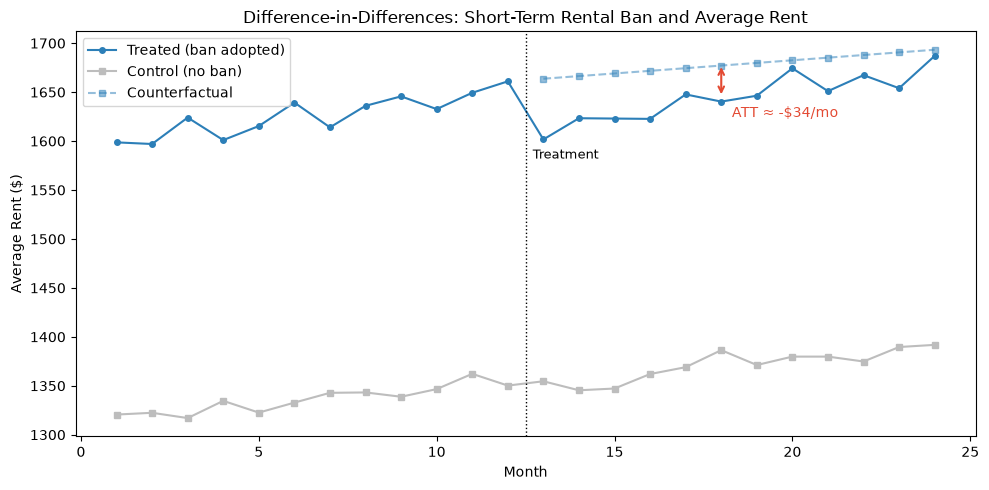
Suppose we wanted to know the effect of a short-term rental ban on average rents. We have eight municipalities, three of which adopted the ban. The simplest approach is to compare treated and control rents after the ban. That post-treatment comparison would suggest the ban increased rents by about $274/month. That number mixes the pre-existing gap between the groups with the ban's actual effect. The treated municipalities already had higher rents before the ban.
Difference-in-differences (DID) accounts for that baseline gap by comparing how much each group changed over the same period. If both groups would have followed the same upward trend without the ban, then the control group's change estimates what the treated group would have done without it. We borrow the control group's trajectory and project it onto the treated group's starting point to estimate the counterfactual. The gap between what we observe and that counterfactual trend is the estimated treatment effect.
DID estimates the ban decreased rents in the affected cities (the ATT) by $34/month. Here is what this looks like in the example data:
DID is mechanically simple, but three assumptions must all hold to recover a valid treatment effect.
- Parallel trends: Both the treatment and control groups follow the same growth trajectory in the absence of treatment. This is the most important assumption of all. If treated cities already had faster-rising rents before the ban, DID would confuse that pre-existing difference in trajectory with the effect of the ban itself. The estimate would no longer isolate the policy effect, but mix the policy with whatever was already making treated cities move differently. We can sanity-check this assumption before treatment.
- No time spillovers: The treatment effect shouldn't bleed into the outcomes of pre-treatment periods. This can happen when interventions are announced in advance. If a short-term rental ban was announced six months in advance, property owners could convert their listings to long-term rentals, flooding the rental market and softening rents before the ban takes effect. That means part of the treatment effect has already happened before the model thinks treatment began, which pushes the estimate toward zero.
- No unit spillovers: This happens if applying an intervention to one unit affects other units. If a ban took place in one city but not in a neighbouring city, investors may pour into the neighbouring city, buy up housing stock, and heat up both purchase and rental prices in the process. That would make the control group's rent growth steeper. The counterfactual for the treated cities would be too high, so the ban would look more rent-reducing than it really was.
DID has many flavours beyond the basic 2x2: versions that incorporate covariates, handle staggered timing, use doubly robust estimation, or estimate dynamic effects over time. Each variant has its own details, but they all try to justify what would have happened to the treated units without treatment.
Synthetic Control
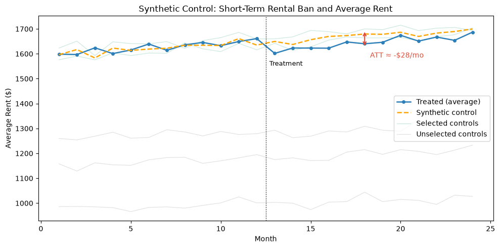
DID compares the treated group to the control group you give it. That can be too blunt when the raw control average is a poor benchmark. It also works poorly with only one or a few treated units. Synthetic Control (SC) handles this by building a custom counterfactual from the controls. Instead of averaging all controls equally, it finds a weighted blend of control units that tracked the treated group as closely as possible before treatment. The post-treatment gap between the treated unit, or treated average, and its synthetic twin is the estimated effect.
Under the hood, this is regression turned sideways. Time periods become the rows and the outcomes of control units become the predictor variables. You fit the model on the pre-treatment period, then use it to impute the treated group's post-treatment counterfactual. The weights are constrained so the synthetic control is a blend of real control units, not an extrapolation built by subtracting one unit from another. If no blend of controls tracked the treated group well before treatment, the post-treatment projection is not trustworthy. You can add covariates to synthetic control, but in many applications the strongest predictors are the pre-treatment outcomes themselves.
SC is often used when there is only one treated unit, but the same idea works for a small treated group. In this example, I'll average the three municipalities that adopted the ban and build a synthetic version of that average. SC estimates an ATT of -$28/month. The blend that produces this synthetic control is 57% Kelowna and 43% Victoria.
Synthetic Difference-in-Differences
DID assumes the treated and control groups share the same growth trajectory. SC requires a weighted blend of controls that closely tracks the treated units before treatment.
Synthetic Difference-in-Differences (SDID) combines both approaches. It uses SC weights to build a better comparison group, then estimates the treatment effect with a DID-style model. Because the DID step absorbs level differences, the synthetic control mainly needs to track the treated group's movement before treatment. The comparison is no longer against the raw untreated group, but against a control group constructed to resemble the treated group before treatment.
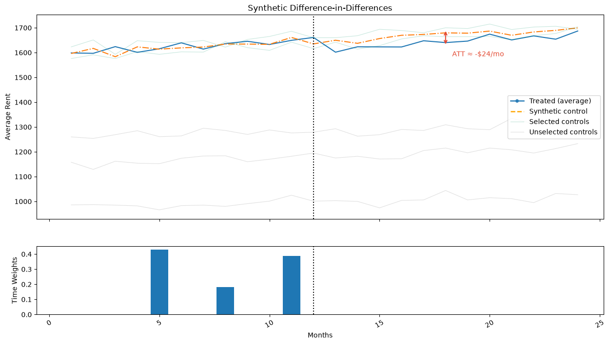
SDID weights both units and time periods. On the unit side, SDID down-weights control cities that tracked the treated group poorly and up-weights the ones that did. On the time side, SDID uses the control cities to learn which pre-treatment months look most like the post-treatment period. Those months get more weight. Traditional DID treats every pre-treatment month equally, but some parts of the pre-treatment period contain more information about the post-treatment period.
In this example, SDID estimates an ATT of -$24/month, assigning all control weight to Kelowna (57%) and Victoria (43%). The three most informative pre-treatment months were months 5, 8, and 11. In this dataset, SC alone already builds a strong counterfactual, so SDID does not dramatically change the estimate. Its value is the more disciplined comparison. The control group is weighted to resemble the treated group, and the DID step handles remaining level differences.
What Difference Does it Make?
Panel methods fill in the treated counterfactual with control information. DID uses the control trend. SC uses a weighted blend of controls. SDID uses both. When the assumptions hold, and that is the hard part, panel methods can estimate aggregate causal effects even without randomization.
These methods answer a different question than the CATE tools from Part 3. They don't tell you which individual city, store, region, or customer responds most to treatment. Rather, they tell you what happened to the treated group on average. With few treated units, the methods sacrifice granularity to build a more credible counterfactual without randomization.