Reading Causal Inference in Python — Part 2: Adjusting for Bias
How to choose control variables for regression and propensity scoring.
AUTHOR
Nathan Horvath
PUBLISHED
2026-05-18
I'm reading Causal Inference in Python by Matheus Facure and writing about its key takeaways I find most useful for applied work. I'm aiming to solidify my existing understanding and help others avoid common pitfalls. You'll want to read my Part 1 post before reading this one!
Most data scientists want more predictive power. Adding variables is the natural move to achieve a better fit. In causal inference, that instinct can destroy your estimate without obvious warning.
Regression doesn't weight groups the way you think it does. The wrong control variable widens your confidence intervals. A propensity model that fits too well can hollow out the identification you're counting on. None of these failures announce themselves.
How Regression Weights Groups
Even with the right variables in your model, regression can still return an estimate that surprises you, because of how it weights groups internally. Most practitioners assume regression combines group effects by sample size. It doesn't. Regression actually weights by within-group treatment variance, the variance left after controlling for the other variables in the model.
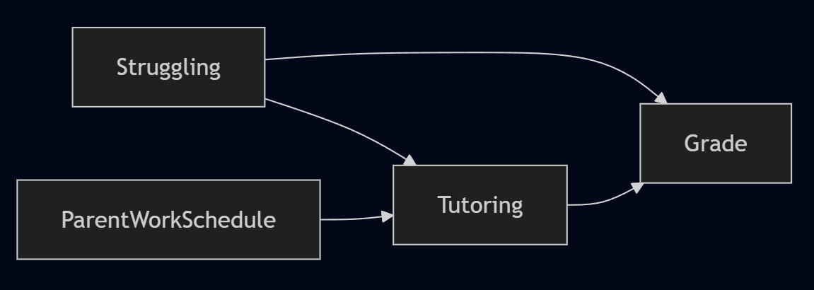
Consider the simple tutoring example from Part 1. Suppose struggling students make up the larger group but receive tutoring at a very high rate, leaving little treatment variation within the group. Non-struggling students are fewer, but their tutoring assignments are more mixed.
| Group | n | Base Grade | True ATE | P(tutoring) |
|---|---|---|---|---|
| Struggling | 200 | 70% | +10% | 90% |
| Non-struggling | 100 | 80% | +2% | 30% |
The simulation below reproduces this setup:
import numpy as np, pandas as pd
import statsmodels.formula.api as smf

np.random.seed(42)
n1, n2 = 200, 100

t1 = np.random.binomial(1, 0.9, n1)
t2 = np.random.binomial(1, 0.3, n2)

df = pd.DataFrame(dict(
    tutoring=np.concatenate([t1, t2]),
    grade=np.concatenate([70 + 10*t1 + np.random.normal(0,3,n1),
                          80 + 2*t2  + np.random.normal(0,3,n2)]),
    group=pd.Categorical(['struggling']*n1 + ['non_struggling']*n2)
))

size_weighted = (10*n1 + 2*n2) / (n1+n2)
regression = smf.ols("grade ~ tutoring + C(group)", data=df).fit().params["tutoring"]
print(f"Sample-size weighted ATE: {size_weighted:.2f}")
print(f"Regression ATE:           {regression:.2f}")
print(f"\nTreatment variance -- struggling: {np.var(t1):.2f}, non-struggling: {np.var(t2):.2f}")
Sample-size weighted ATE: 7.33
Regression ATE:           5.50

Treatment variance -- struggling: 0.09, non-struggling: 0.21
Regression, controlling for group, returns an ATE estimate of +5.50%. The non-struggling group has half the sample size, but its larger treatment variance (0.21 compared to 0.09) gives it more influence over the combined estimate, pulling the result down from the sample-size-weighted average of +7.33% to +5.50%.
So which variables should you actually be controlling for in regression? To answer that, you need to understand what regression is doing under the hood.
When More Variables Backfire in Regression
The instinct when building a causal model is to include every variable. In prediction, that's often desirable. In causal inference, the wrong variable can make a real effect vanish into noise. The Frisch-Waugh-Lovell (FWL) theorem explains why.
FWL shows that multivariate regression is doing two separate jobs at once. The first is debiasing: regress treatment $T$ on confounders $X$, take the residuals $\tilde{T}$, and you get the part of treatment variation the confounders can't explain. The second is denoising: regress outcome $Y$ on the same confounders, take those residuals $\tilde{Y}$, and you get the part of outcome variation the confounders can't explain. Debiasing removes confounding bias and is required. Denoising reduces variance and is optional, but generally desired. FWL accounts for the variance-weighting result from the previous section. Groups with more residual treatment variation in $\tilde{T}$ contribute more to the final estimate, which is why the non-struggling group exerted disproportionate influence despite its smaller size.
In the original Part 1 example, struggling students are more likely to seek tutoring and perform worse regardless, so Struggling has arrows to both the treatment (Tutoring) and outcome (Grade). Including it closes a backdoor path and reduces bias. That's a true confounder and it belongs in the model.
Now consider a second variable: parent work schedules. Busy parents have less time to arrange tutoring sessions, so this variable has an arrow to Tutoring. But a parent's work schedule doesn't directly impact grades, so there's no arrow to Grade.
The catch is that regression performs both steps with the same set of variables. When you add Parent Work Schedule, regression residualizes $T$ on it as part of the debiasing step, absorbing variation that had nothing to do with confounding. Less of $\tilde{T}$ remains, and your causal estimate is built on a narrower base of information. Confidence intervals widen, sometimes enough to mask a real effect entirely. Adding the wrong variable is a self-inflicted wound.
The opposite case is a variable that affects the outcome $Y$ but not the treatment $T$, such as access to a quiet study space. This cleans up residual noise in $Y$ without touching $\tilde{T}$, tightening your estimate. Regression has no way to treat these two cases differently. Other modeling approaches, like Double Machine Learning (to be covered in Part 3), allow you to decompose these steps explicitly and assign variables where they actually help.
The Propensity Score Trap
Propensity score modeling shares the same variable selection problem, but the trap is different and harder to detect. In regression, the damage shows up in your standard errors. In propensity scoring, a poor causal estimate hides behind a model that looks increasingly impressive.
With observational data, some units ended up in the treated group because of their covariate profile, not by chance. To debias the analysis, Inverse Propensity Weighting (IPW) up-weights the units that look like they were assigned contrary to what their covariates would predict. A treated unit whose covariates resemble the control group tells you what treatment does to people who wouldn't normally get it. A control unit whose covariates resemble the treated group tells you what withholding treatment does to people who would normally receive it. These "surprising" assignments are where the identification comes from.
To identify these "surprising" units, you need a propensity model. The trap occurs when you include variables strongly linked to treatment but with little connection to the outcome. Yes, those variables make the model better at separating treated from control, but that separation erodes overlap without reducing any bias.
As the model improves at separating groups, units that received the "wrong" treatment become increasingly rare. The few that remain land near the extremes: treated units with very low propensity scores, control units with very high ones. IPW weights these by the inverse of their propensity scores, so as extreme units grow rarer, the weights on the remaining extreme units grow larger. Eventually a handful of observations dominates the entire estimate, and variance climbs with them.
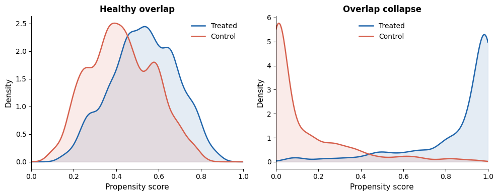
Left: treated and control units mix across the full range of propensity scores. Right: a stronger treatment model pulls them apart, and the "surprising" assignments IPW needs disappear.
When the model gets good enough, every treated unit ends up with a high score and every control unit with a low score. No units cross the middle. Without treated units in the low-propensity region and control units in the high-propensity region, there are no surprising assignments left to up-weight. Model performance metrics look great. The causal estimate subtly falls apart.
A model that perfectly separates treated from control is the worst possible model for causal estimation. The variables that belong are confounders, as omitting them creates bias. Choosing which variables belong is what separates a useful causal estimate from a confident wrong answer.
The Method is the Easy Part
Picking the estimator is the easy part. The literature has plenty of methods to choose from. None of them will flag when you've fed them the wrong inputs. If you can randomize, you probably should. When you can't, the work is in understanding what each variable is actually doing in your model before you add it. That's not something you can automate away.